Time Series Models

1 Introduction

The tsarma package implements methods for the estimation, inference, filtering, prediction and simulation of stationary time series using the ARMA(p,q)-X model. It makes use of the tsmodels framework, providing common methods with similar inputs and classes with similar outputs.

The Appendix provides a table with a hierarchical overview of the main functions and methods currently implemented in the package.

2 Estimation

The ARMA(p,q)-X model implemented in the package has the following representation:

\[ \Phi\left(L\right)\left(1-L\right)\left(y_t - \mu_t\right) = \Theta\left(L\right)\varepsilon_t \tag{1}\]

where $L$ is the lag operator. This can equivalently be written out as:

\[ \begin{aligned} \mu_t &= \mu + \sum^k_{j=1}\xi_jx_t\\ y_t &= \mu_t + \sum^p_{j=1}\phi_j \left(y_{t-j} - \mu_{t-j}\right) + \sum^q_{j=1}\theta_j\varepsilon_{t-j} + \varepsilon_t\\ \varepsilon_t &\sim D\left(0, \sigma,\ldots\right) \end{aligned} \tag{2}\]

where $x$ is an optional matrix of external pre-lagged regressors with coefficients $\xi$. The ARMA coefficients are $\phi$ and $\theta$ respectively, constrained during estimation so that their inverse roots are less than unity. The residuals $\varepsilon_t$ can be modeled using one of the distributions implemented in the tsdistributions package with additional parameters ($\ldots$) to capture higher order moments. Both $\mu$ and $\sigma$ are estimated, not concentrated out.

Initialization of the ARMA recursion proceeds as follows:

For a ARMA(p,q) or ARMA (p,0) model with $p > 0$, the recursion is initialized at time $t=p+1$ so that p degrees of freedom are used up. If an MA term is present ($q>0$), then it will also be initialized at time $t=p+1$ irrespective of the MA order, allowing all terms in the MA component ($j=\left(1,\ldots,q\right)$) for which $t>j$ to contribute to the initial fitted values.
For an ARMA(0,q) model with $q>0$, the recursion is initialized at time $t=2$ allowing all terms in the MA component ($j=\left(1,\ldots,q\right)$) for which $t>j$ to contribute to the initial fitted values.

Initial values for the coefficients proceed by first trying a pass through the stats::arima function, and if that fails, then then the method of Hannan and Rissanen (1982) is used instead.

Estimation uses the nloptr solver with analytic gradients provided through the use of the TMB package for which a custom C++ functions have been created written to minimize the log-likelihood subject to the distribution chosen. Inequality constraints for stationarity (AR) and invertibility (MA) are imposed and their Jacobians calculated using jacobian function from the the numDeriv package.

Standard errors are implemented with methods for bread and estfun (scores), in addition to functions for meat and meat_HAC using the sandwich package framework.

3 Demonstration

3.1 Estimation

We demonstrate the functionality of the package using the SPY ETF price series from the tsdatasets package using an ARMA(2,1) model, after taking log differences.

Code

spy <- tsdatasets::spy
spyr <- diff(log(spy$Close))[-1]
spec <- arma_modelspec(spyr[1:2000], order = c(2,1), distribution = "jsu")
mod <- estimate(spec)
summary(mod, vcov_type = "QMLE")

ARMA Model Summary

Coefficients:
         Estimate Std. Error t value Pr(>|t|)    
mu      0.0006270  0.0001698   3.691 0.000223 ***
phi1    0.6761683  0.0856419   7.895 2.89e-15 ***
phi2   -0.0483387  0.0309519  -1.562 0.118350    
theta1 -0.7325296  0.0855267  -8.565  < 2e-16 ***
sigma   0.0107081  0.0003383  31.656  < 2e-16 ***
skew   -0.1140090  0.0520472  -2.190 0.028489 *  
shape   1.2222210  0.0632283  19.330  < 2e-16 ***
---
Signif. codes:  0 '***' 0.001 '**' 0.01 '*' 0.05 '.' 0.1 ' ' 1

N =  2000
LogLik =  6446,  AIC =   -12880,  BIC =  -12840

The summary method has an optional argument for the type of coefficient covariance matrix to use for calculating the standard errors. Valid options are the analytic hessian (“H”), outer product of gradients (“OP”), Quasi-MLE (“QMLE”) and Newey-West (“NW”) for which additional arguments can be passed (see the bwNeweyWest function in the sandwich package).

A nicer table can be generated using the as_flextable method, which we illustrate below:

Code

model_summary <- summary(mod, vcov_type = "QMLE")
out <- as_flextable(model_summary, table.caption = "SPY ARMA(2,1)~JSU")
out


	Estimate	Std. Error	t value	Pr(>\|t\|)
$\mu$	0.0006	0.0002	3.6914	0.0002	***
$\phi_1$	0.6762	0.0856	7.8953	0.0000	***
$\phi_2$	-0.0483	0.0310	-1.5617	0.1184
$\theta_1$	-0.7325	0.0855	-8.5649	0.0000	***
$\sigma$	0.0107	0.0003	31.6563	0.0000	***
$\zeta$	-0.1140	0.0520	-2.1905	0.0285	*
$\nu$	1.2222	0.0632	19.3303	0.0000	***
Signif. codes: 0 '*' 0.001 '' 0.01 '*' 0.05 '.' 0.1 ' ' 1
LogLik = 6446
AIC = -12878 , BIC = -12838

Model Equation $\mu_t = \mu$
$\hat y_t = \mu_t + \sum_{j=1}^2\phi_j \left(y_{t-j}-\mu_{t-j}\right) + \theta_1\varepsilon_{t-1} + \varepsilon_t$ $\varepsilon_t \sim JSU\left(0,\sigma,\zeta, \nu\right)$

There are options to control what goes into the table and whether parameters should be kept with their names or symbols. The model equation is generated from the tsequation method.

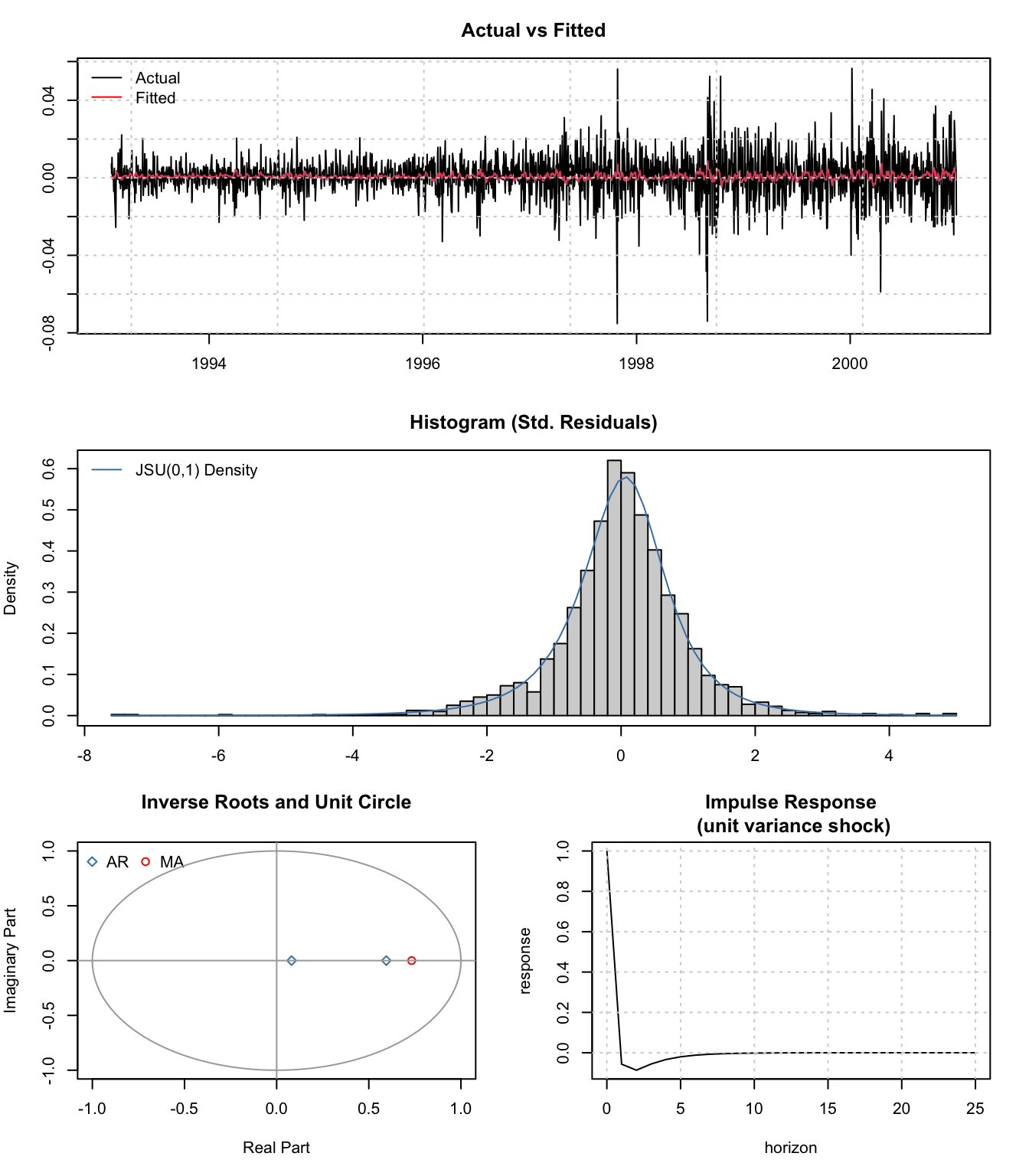
The plot method on the estimated object generates a set of 4 plots of the fitted against actual values, the histogram of the standardized residuals against the expected density of the distribution used, and the ARMA inverse roots and impulse response function.

Code

plot(mod)

The impulse response function (arma_irf) of this model shows that a unit variance shock will decay to zero after about 5 periods.

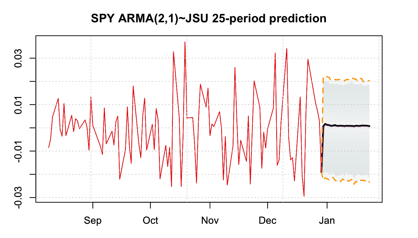
3.2 Prediction

The predict method will generate h step ahead predictions of the conditional mean, the model standard deviation as well as a simulated predictive distribution using either bootstrap re-sampling of the residuals else parametric sampling based on the distribution chosen to estimate the model. Optionally, the user can pass in a matrix of innovations to be used instead. These can either be uniform deviates (in effect quantiles) which will be transformed into the model’s distributional innovations, standardized innovations which will be scaled by the standard deviation of the model, else non-standardized innovations. The latter may be useful when passing a GARCH generated set of forecast innovations.

The forc_dates argument allows the user to pass a set of time indices representing the forecast horizon, else the function will try to auto-generate these based on the estimated sampling frequency of the data.

Code

p <- predict(mod, h = 25, bootstrap = TRUE, nsim = 5000)
head(cbind(p$mean, p$sigma))

                 p.mean    p.sigma
2000-12-30 0.0004112512 0.01070811
2000-12-31 0.0014352212 0.01072511
2001-01-01 0.0011839164 0.01076498
2001-01-02 0.0009644945 0.01078151
2001-01-03 0.0008282762 0.01078748
2001-01-04 0.0007467763 0.01078959

The variance of the prediction error at time $t+h$ is equal to:

\[ \hat \sigma\sum^{h-1}_{i=0}\Psi^2_i \tag{3}\]

where $\Psi$ represent the infinite MA representation of an ARMA(p,q) model (psi-weights), which can be generated using the stats::ARMAtoMA function.

Since the output is of class tsmodel.predict, the corresponding plot method from the tsmethods package can be used directly.

Code

par(mar = c(3,3,3,3))
plot(p, n_original = 100, main = "SPY ARMA(2,1)~JSU 25-period prediction", ylab = "", xlab = "", gradient_color = "azure3",interval_color = "orange")

3.3 Filtering and Simulation

The 2 final methods of note in the package are tsfilter and simulate which allow the filtering of new data and simulation, respectively. Both of these methods can be dispatched from either an estimated model of class tsarma.estimate as well as a specification object of class tsarma.spec. In the following demonstration, the combination of tsfilter and simulate methods is illustrated.

We first take the original specification object and replace the parameter matrix holding the estimated parameters from the estimated object. This is all that is required.

Code

parmatrix <- copy(mod$parmatrix)
spec$parmatrix <- parmatrix

In the next step we verify that tsfilter both the specification and estimated objects return the same result.

Code

filter_spec <- tsfilter(spec, y = spyr[2001:2010])
filter_model <- tsfilter(mod, y = spyr[2001:2010])
all.equal(fitted(filter_spec), fitted(filter_model))

[1] TRUE

Filtering on a specification object is equivalent to running through the ARMA recursion with fixed parameters. We can check that passing a specification object without new data to tsfilter will results in the same values as those from the estimated model.

Code

filter_spec <- tsfilter(spec)
all.equal(fitted(mod), fitted(filter_spec))

[1] TRUE

It is also possible to completely replace y with a new dataset if we have pooled estimates of the parameters to use in the parameter matrix. Simply put, the filtering algorithm takes a set of fixed parameters and filters the data.

Next, we illustrate how to generate a predictive distribution using the simulate method on both the estimated and specification objects and verify replication of results with the predict method.

Code

sim_spec <- spec
sim_spec$parmatrix <- copy(mod$parmatrix)
filter_spec <- tsfilter(sim_spec)
maxpq <- max(spec$model$order)
series_init <- tail(sim_spec$target$y_orig, maxpq)
innov_init <- as.numeric(tail(residuals(filter_spec), maxpq))
simulate_spec <- simulate(sim_spec, nsim = 2000, seed = 100, h = 10, series_init = series_init, innov_init = innov_init)
simulate_model <- simulate(mod, nsim = 2000, seed = 100, h = 10, series_init = series_init, innov_init = innov_init)
set.seed(100)
p <- predict(mod, h = 10, nsim = 2000)
# equivalence between estimation and specification simulated distributions
all.equal(simulate_spec$simulated, simulate_model$simulated)

[1] TRUE

Code

# equivalence between simulation method and prediction method distributions
all.equal(simulate_spec$simulated, p$distribution)

[1] TRUE

4 Conclusion

The tsarma package is currently under development and may change in the future. Potential areas for improvement are likely to be the inclusion of non-stationary series turning it into an ARIMA model. Adding seasonality is not something which is planned, and users who work with stationary seasonal series can use fourier terms in the regressors using the fourier_series function from tsaux.

5 Appendix

5.1 Methods and Classes


(...)	type	input	output
tsarma
¦--arma_modelspec	function	xts	tsarma.spec
¦ ¦--simulate	method	tsarma.spec	tsarma.simulate
¦ ¦--tsfilter	method	tsarma.spec	tsarma.estimate
¦ °--tsbacktest	method	tsarma.spec	list
¦--estimate	method	tsarma.spec	tsarma.estimate
¦ ¦--summary	method	tsarma.estimate	summary.tsarma
¦ ¦ °--print	method	summary.tsarma	print/flextable
¦ ¦--tidy	method	tsarma.estimate	tibble
¦ ¦--glance	method	tsarma.estimate	tibble
¦ ¦--plot	method	tsarma.estimate	plot
¦ ¦--coef	method	tsarma.estimate	numeric
¦ ¦--logLik	method	tsarma.estimate	logLik
¦ ¦--fitted	method	tsarma.estimate	xts
¦ ¦--residuals	method	tsarma.estimate	xts
¦ ¦--tsequation	method	tsarma.estimate	list
¦ ¦--AIC	method	tsarma.estimate	numeric
¦ ¦--BIC	method	tsarma.estimate	numeric
¦ ¦--confint	method	tsarma.estimate	matrix
¦ ¦--vcov	method	tsarma.estimate	matrix
¦ ¦--bread	method	tsarma.estimate	matrix
¦ ¦--estfun	method	tsarma.estimate	matrix
¦ ¦--predict	method	tsarma.estimate	tsmodel.predict
¦ ¦ ¦--plot	method	tsmodel.predict	plot
¦ ¦ °--pit	method	tsarma.predict	xts
¦ ¦--simulate	method	tsarma.estimate	tsmodel.simulate
¦ ¦--tsfilter	method	tsarma.estimate	tsmodel.estimate
¦ ¦--unconditional	method	tsarma.estimate	numeric
¦ ¦--sigma	method	tsarma.estimate	numeric
¦ ¦--nobs	method	tsarma.estimate	numeric
¦ ¦--pit	method	tsarma.estimate	xts
¦ °--halflife	method	numeric	numeric
¦--arma_irf	function	numeric	arma.irf
¦ °--plot	method	arma.irf	plot
°--arma_roots	function	numeric	arma.roots
°--plot	method	arma.roots	plot

6 References

Hannan, Edward J, and Jorma Rissanen, 1982, Recursive estimation of mixed autoregressive-moving average order, Biometrika 69, 81–94.