A short demo on generating the authorized domain of a distribution.
distributions
tsdistributions
Author
Alexios Galanos
Published
May 11, 2022
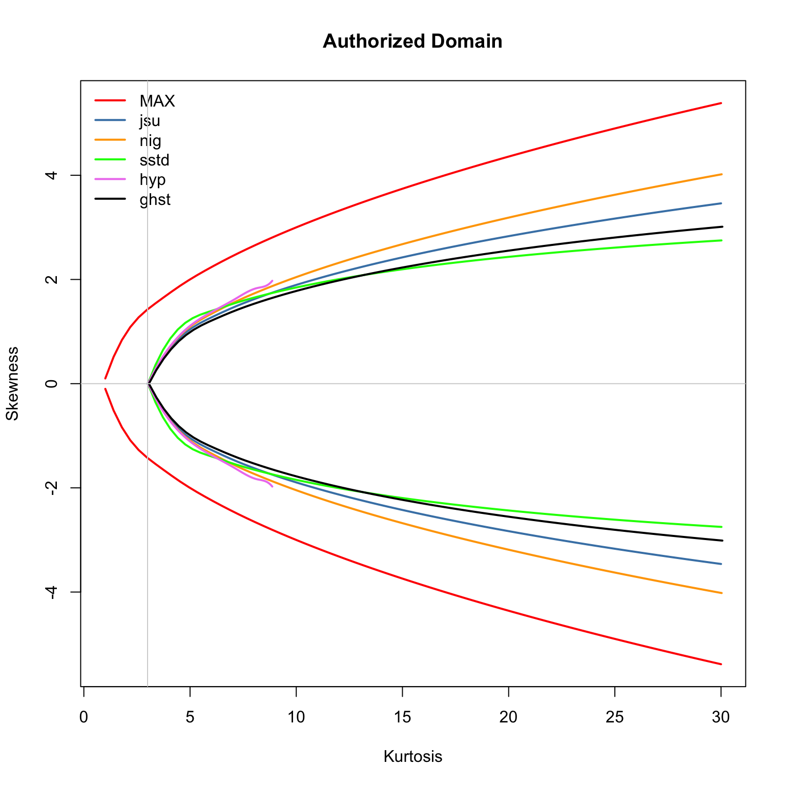
The tsdistributions package provides the function authorized_domain which calculates the region of Skewness-Kurtosis for which a density exists. This is related to the Hamburger moment problem, and the maximum attainable Skewness (S) given kurtosis (K) (see (Widder 2015)). A key takeaway from Widder is that for as given level of kurtosis(\(\mu_4\)) only a finite range of skewness (\(\mu_3\)) may be attained, with the boundary given by:
This short demo shows how to generate a plot comparing a number of different skewed and heavy tailed distributions available in the package. We investigate Johnson’s SU (jsu), the Normal Inverse Gaussian (nig), the Skew Student of Fernandez and Steel (sstd), the Hyperbolic and the Generalized Hyperbolic Skewed Student (ghst) distributions.
Code
library(tsdistributions)# default is maximum kurtosis of 30 with interval length of 25max_kurt <-30n <-25jsud <-authorized_domain("jsu", max_kurt = max_kurt, n = n)nigd <-authorized_domain("nig")sstdd <-authorized_domain("sstd")ghypd <-authorized_domain("gh", lambda =1)ghstd <-authorized_domain("ghst")
The returned list contains the lower half of the Skewness-Kurtosis combinations, so we reflect those values to obtain the upper half and plot them. The curves delimit the skewness-kurtosis boundary corresponding to the authorized domain, for which a density exists.
Code
K =c(seq(1.01, max_kurt, length.out = n), seq(1.01, max_kurt, length.out = n))S =c(sqrt(seq(1.01, max_kurt, length.out = n) -1), -sqrt(seq(1.01, max_kurt, length.out = n) -1))plot(K, S, ylab ="Skewness", xlab ="Kurtosis", main ="Authorized Domain", type ="n")lines(spline(K[1:n], S[1:n]), col ="red", lwd =2)lines(spline(K[1:n], -S[1:n]), col ="red" ,lwd =2)lines(jsud$Kurtosis, jsud$Skewness, col ="steelblue", lwd =2)lines(jsud$Kurtosis, -jsud$Skewness, col ="steelblue", lwd =2)lines(nigd$Kurtosis, nigd$Skewness, col ="orange", lwd =2)lines(nigd$Kurtosis, -nigd$Skewness, col ="orange", lwd =2)lines(sstdd$Kurtosis, sstdd$Skewness, col ="green", lwd =2)lines(sstdd$Kurtosis, -sstdd$Skewness, col ="green", lwd =2)lines(ghypd$Kurtosis, ghypd$Skewness, col ="violet", lwd =2)lines(ghypd$Kurtosis, -ghypd$Skewness, col ="violet", lwd =2)lines(ghstd$Kurtosis, ghstd$Skewness, col ="black", lwd =2)lines(ghstd$Kurtosis, -ghstd$Skewness, col ="black", lwd =2)legend("topleft", c("MAX", "jsu","nig","sstd","hyp","ghst"), col =c("red", "steelblue","orange","green","violet","black"), lty =1, lwd =rep(2, 5), bty ="n")abline(v =3, col ="lightgrey")abline(h =0, col ="lightgrey")