Tails of the GHST

We take a closer look at the properties of the GHST distribution which uniquely, in the family of Generalized Hyperbolic distributions, can accomodate one heavy and one semi-heavy tail.

distributions
tsdistributions
Author

Alexios Galanos

Published

May 12, 2022

Code
library(tsdistributions)
library(data.table)
assignInNamespace("cedta.override", c(data.table:::cedta.override,"distill"), "data.table")
library(ggplot2)
library(gridExtra)
f1 <- function(x) ddist("ghst", x, 2, 1, skew = -20, shape = 10)
f2 <- function(x) ddist("ghst", x, -2, 1, skew = 20, shape = 10)
ggplot(NULL, aes(c(-6,6))) + 
  geom_area(stat = "function", fun = f1, fill = "cadetblue", alpha = 0.4, xlim = c(-6, 6)) + 
  geom_area(stat = "function", fun = f2, fill = "darkgrey", alpha = 0.4, xlim = c(-6, 6))  + 
  ggthemes::theme_tufte() + 
  xlab("") + 
  ylab("") + 
  ggtitle("The GHST")

Introduction

The Generalized Hyperbolic Skew Student distribution, described in (Aas and Haff 2006), is a sub-family of the Generalized Hyperbolic distribution of (Barndorff-Nielsen 1977). It has the unique property of allowing the 2 tails to exhibit different behaviors, namely one polynomial and one exponential. This is important in some applications such as financial time series where negative shocks exhibit heavy tails, whereas positive shocks have a more Gaussian type tail.

Tail Behavior

This distribution is a limiting case of the Generalized Hyperbolic when \(\alpha \to \left| \beta \right|\) and \(\lambda=-\nu/2\), where \(\nu\) is the shape parameter of the Student distribution. The domain of variation of the parameters is \(\beta \in \mathbb{R}\) and \(\nu>0\), but for the variance to be finite \(\nu>4\), while for the existence of skewness and kurtosis, \(\nu>6\) and \(\nu>8\) respectively.

Following (Aas and Haff 2006), the heaviest tail decays as:

\[ f_x(x) \sim \text{const}|x|^{-\nu/{2-1}}\quad \text{when} \begin{cases} \beta <0 \quad and \quad x\rightarrow -\infty & \\ \beta >0 \quad and \quad x\rightarrow +\infty & \\ \end{cases} \tag{1}\]

and the semi-heavy tail decays as:

\[ f_x(x) \sim \text{const}|x|^{-\nu/{2-1}}\text{exp}\left(-2|\beta x|\right)\quad \text{when} \begin{cases} \beta <0 \quad and \quad x\rightarrow +\infty & \\ \beta >0 \quad and \quad x\rightarrow -\infty & \\ \end{cases} \tag{2}\]

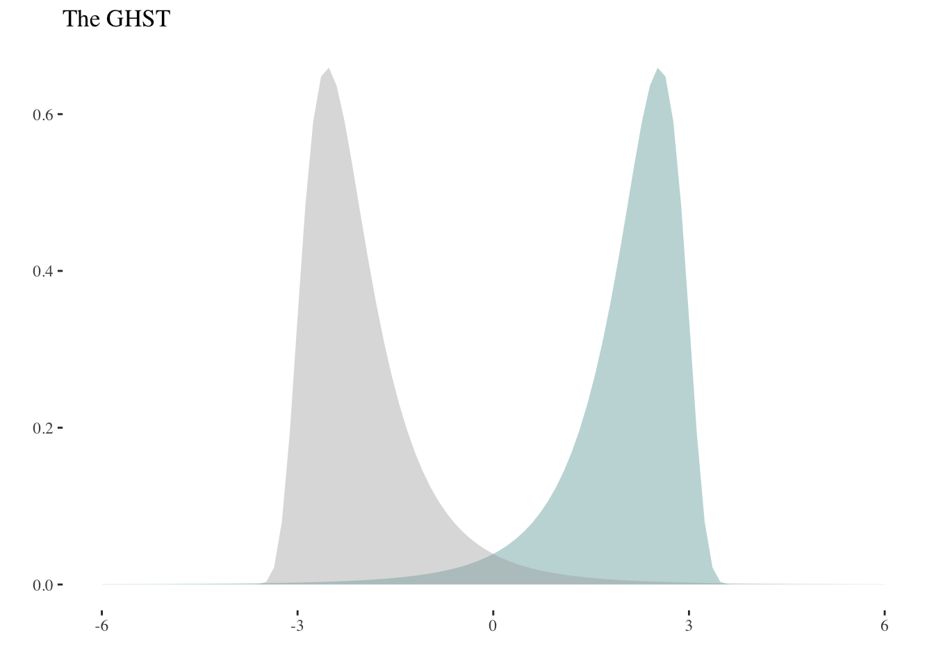
The skew and shape parameters of the standardized parameterization in the tsdistributions have bounds \(\in\{-\infty, +\infty\}\) and \(\in R^+\) respectively. The further the skew parameter is from zero and the smaller the shape parameter is, the larger the skewness. The plot below illustrates an example of the tail behavior that can be generated from this distribution.

Code
library(tsdistributions)
library(data.table)
library(ggplot2)
f1 <- function(x) ddist("ghst", x, 0, 1, skew = -30, shape = 30)
f2 <- function(x) ddist("ghst", x, 0, 1, skew = -30, shape = 10)
ggplot(NULL, aes(c(-6,6))) + 
  geom_area(aes(colour = "plotA", fill = "plotA"), stat = "function", fun = f1, fill = "orange", alpha = 0.4, xlim = c(-6, 6)) + 
  geom_area(aes(colour = "plotB", fill = "plotB"), stat = "function", fun = f2, fill = "steelblue", alpha = 0.4, xlim = c(-6, 6)) +
  ggthemes::theme_tufte() + xlab("") + 
  ylab("") + 
  ggtitle("The GHST") + 
  theme(legend.position = "right") + 
  scale_fill_manual(name = " ", values =  c(plotA = "orange", plotB = "steelblue"), aesthetics = c("colour","fill"),
                    labels = c("{skew = -30, shape = 30}","{skew = -30, shape = 10}"))

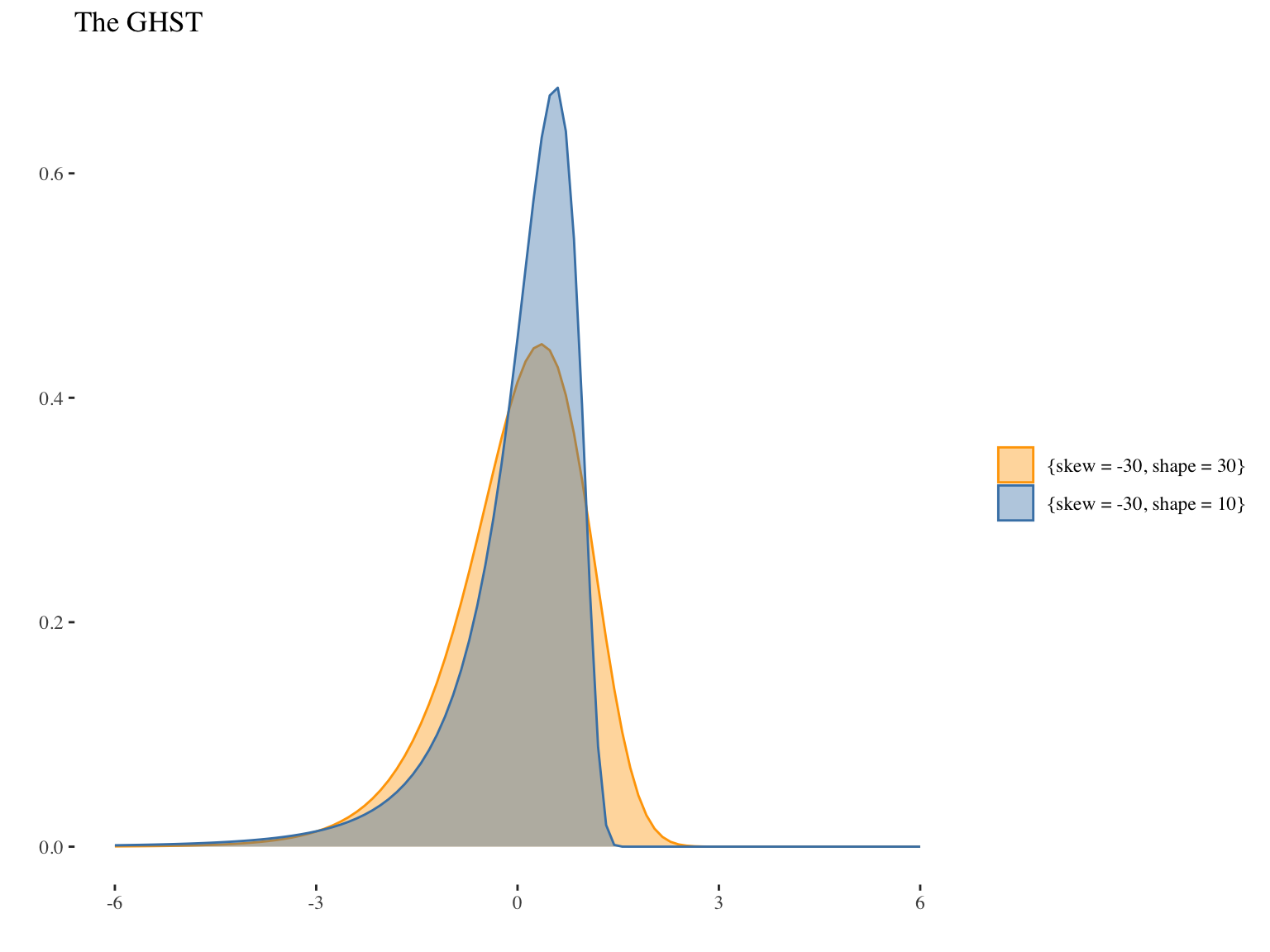
With a skew parameter of -30 common across both, the orange distribution has a shape parameter of 30 with skewness and excess kurtosis of (-0.92, 1.9) while the blue distribution has a shape parameter of 10 with skewness and excess kurtosis of (-3.37, 40.15). For the blue distribution (with the lower shape parameter) the lower heavy and upper semi-heavy tails are quite obvious and hopefully illustrate the value of this distributions for a number of possible applications.

Parameter Distribution and Consistency

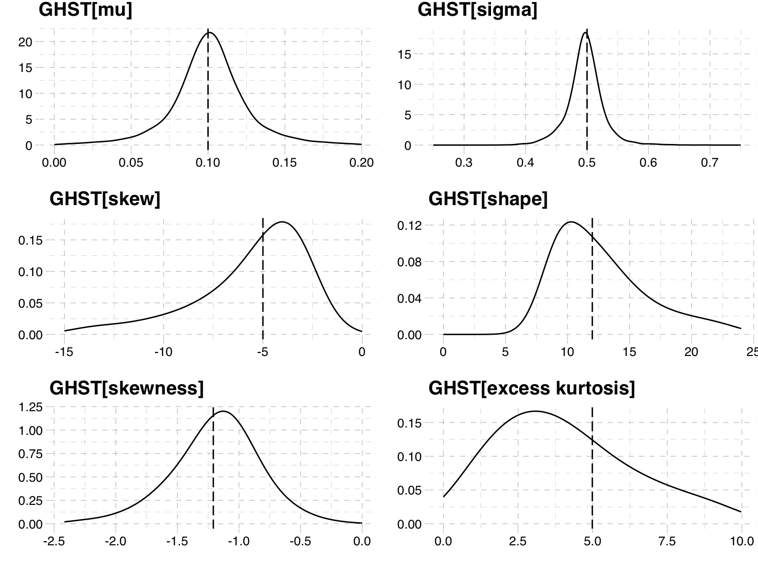
The question of how much data (size) is needed to confidently estimate the true parameter values is one we address here through a small simulation exercise.

Let’s assume that that the true parameters are given \(\mu = 0.1\), \(\sigma = 0.5\), \(\text{skew} = -5\) and \(\text{shape} = 12\). We simulate 2000 draws from sizes of 100, 200, 400, 800, 1200, 1600, 3200 and estimate their parameters. In order to ensure the existence of the higher moments, we also set a lower bound for the shape parameter at 9 and use parallel computation to speed things up.

Code
library(future.apply)
plan(list(
    tweak(remote, workers = "home_server"),
    tweak(multisession, workers = 100)
))
pars %<-% future_lapply(X = 1:2000, function(i){
  r <- rdist("ghst", n = 3200, mu = 0.1, sigma = 0.5, skew = -5, shape = 12)
  sim_lengths <- c(100, 200, 400, 800, 1200, 1600, 3200)
  x <- lapply(sim_lengths, function(j){
   spec <- distribution_modelspec(r[1:j], "ghst")
   spec$parmatrix[parameter == "shape", lower := 9]
   mod <- try(estimate(spec), silent = TRUE)
   if (inherits(mod, "try-error")) {
    v <- rep(as.numeric(NA), 4)
    .skewness <- as.numeric(NA)
    .kurtosis <- as.numeric(NA)
   } else {
    v <- coef(mod)
    .skewness <- dskewness("ghst", skew = v[3], shape = v[4])
    .kurtosis <- dkurtosis("ghst", skew = v[3], shape = v[4])
   }
   return(data.table(sim = i, size = j, mu = as.numeric(v[1]), sigma = as.numeric(v[2]), 
                     skew = as.numeric(v[3]), shape = as.numeric(v[4]),
                     skewness = .skewness, kurtosis = .kurtosis))
  })
  x <- rbindlist(x)
  return(x)
}, future.packages = c("data.table","tsdistributions","tsmethods"), future.seed = TRUE)
pars <- eval(pars)
pars <- rbindlist(pars)
pars <- pars[!is.na(mu)]
plan(sequential)

Parameter Distribution Plots

Code
p1 <- ggplot(pars, aes(mu, fill = size, colour = size)) + 
  xlim(0, 0.2) +
  geom_density(alpha = 0.1, adjust = 2) + 
  geom_vline(xintercept = 0.1, colour = "black", linetype = "longdash") + 
  labs(title = "GHST[mu]") + 
  ylab("") + 
  xlab("") + 
  ggthemes::theme_pander()
p2 <- ggplot(pars, aes(sigma, fill = size, colour = size)) + 
  xlim(0.25, 0.75) +
  geom_density(alpha = 0.1, adjust = 2) + 
  geom_vline(xintercept = 0.5, colour = "black", linetype = "longdash") + 
  labs(title = "GHST[sigma]") + 
  ylab("") + 
  xlab("") + 
  ggthemes::theme_pander()
p3 <- ggplot(pars, aes(skew, fill = size, colour = size)) + 
  xlim(-15, 0) +
  geom_density(alpha = 0.1, adjust = 3) + 
  geom_vline(xintercept = -5, colour = "black", linetype = "longdash") + 
  labs(title = "GHST[skew]") + 
  ylab("") + 
  xlab("") + 
  ggthemes::theme_pander()
p4 <- ggplot(pars, aes(shape, fill = size, colour = size)) + 
  xlim(0, 24) + 
  geom_density(alpha = 0.1, adjust = 3) + 
  geom_vline(xintercept = 12, colour = "black", linetype = "longdash") + 
  labs(title = "GHST[shape]") + 
  ylab("") + 
  xlab("") + 
  ggthemes::theme_pander()
exact_skewness <- dskewness("ghst", skew = -5, shape = 12)
exact_kurtosis <- dkurtosis("ghst", skew = -5, shape = 12)
p5 <- ggplot(pars, aes(skewness, fill = size, colour = size)) + 
  xlim(exact_skewness * 2, 0) + 
  geom_density(alpha = 0.1, adjust = 3) + 
  geom_vline(xintercept = exact_skewness, colour = "black", linetype = "longdash") + 
  labs(title = "GHST[skewness]") + 
  ylab("") + 
  xlab("") + 
  ggthemes::theme_pander()
p6 <- ggplot(pars, aes(kurtosis, fill = size, colour = size)) + 
  xlim(0, exact_kurtosis * 2) +
  geom_density(alpha = 0.1, adjust = 3) +  
  geom_vline(xintercept = exact_kurtosis, colour = "black", linetype = "longdash") + 
  labs(title = "GHST[excess kurtosis]") + 
  ylab("") + 
  xlab("") + 
  ggthemes::theme_pander()
grid.arrange(p1,p2,p3,p4,p5,p6, nrow = 3, ncol = 2)

Size and MAPE Plots

The following plots show the mean absolute percent error per window size for some of the parameters.

Code
skew_mape <- pars[,list(mape = mean(abs((skew - -5)/(-5)))), by = "size"]
p3 <- ggplot(skew_mape, aes(y = mape, x = size)) + geom_line() + 
  labs(title = "GHST[skew]") + 
  xlab("") +  ylab("") + 
  scale_y_continuous(labels = scales::percent)
shape_mape <- pars[,list(mape = mean(abs((shape - 12)/12))), by = "size"]
p4 <- ggplot(shape_mape, aes(y = mape, x = as.numeric(size))) + geom_line() + 
  labs(title = "GHST[shape]") + 
  xlab("") +  ylab("") + 
  scale_y_continuous(labels = scales::percent)
skewness_mape <- pars[,list(mape = mean(abs((skewness - exact_skewness)/exact_skewness))), by = "size"]
p5 <- ggplot(skewness_mape, aes(y = mape, x = as.numeric(size))) + geom_line() + 
  labs(title = "GHST[skewness]") + 
  xlab("") +  ylab("") + 
  scale_y_continuous(labels = scales::percent)
kurtosis_mape <- pars[,list(mape = mean(abs((kurtosis - exact_kurtosis)/exact_kurtosis))), by = "size"]
p6 <- ggplot(kurtosis_mape, aes(y = mape, x = as.numeric(size))) + geom_line() + 
  labs(title = "GHST[excess kurtosis]") + 
  xlab("") + ylab("") + 
  scale_y_continuous(labels = scales::percent) 
grid.arrange(p3,p4,p5,p6, nrow = 2, ncol = 2)

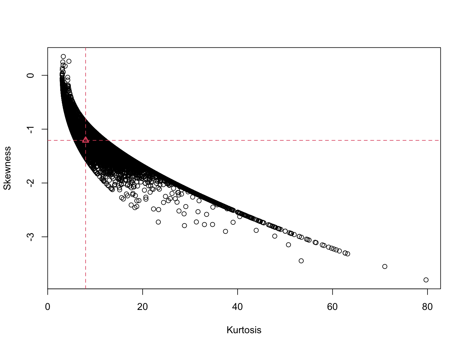
Another interesting plot is that of Kurtosis1 against Skewness.

Code
plot(pars$kurtosis + 3, pars$skewness, ylab = "Skewness", xlab = "Kurtosis")
abline(v = exact_kurtosis + 3, h = exact_skewness, col = 2, lty = 2)
points(exact_kurtosis + 3, exact_skewness, pch = 2, lwd = 2, col = 2)

Final Thoughts

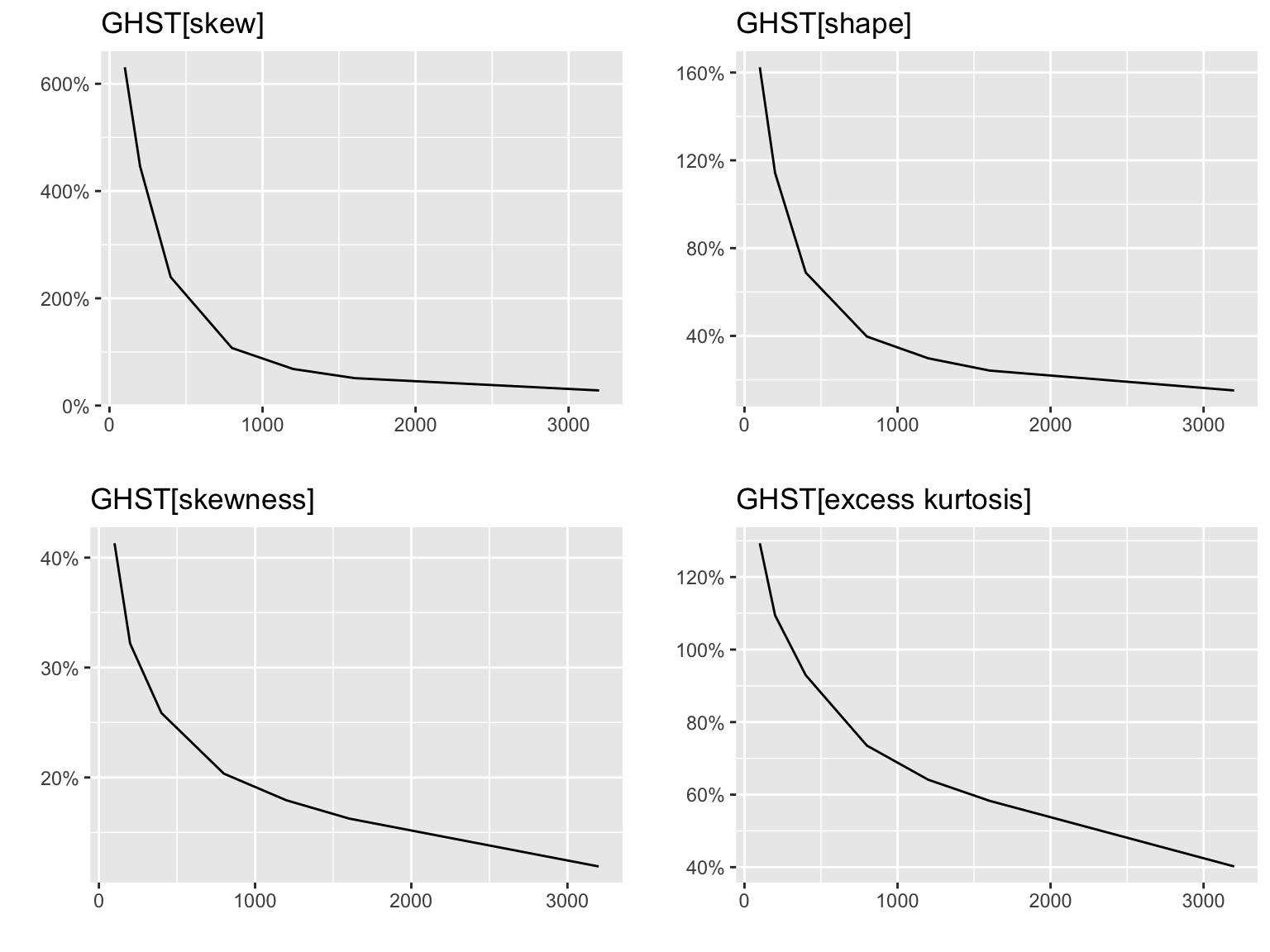
The GHST distribution has some interesting properties, but we also found that a considerable amount of data is needed to provide confident estimates of the higher moments, and we suspect this gets worse the lower the shape parameter is. This could also be due to the fact that our estimation code makes use of the modified Bessel function of the second kind for which the derivatives are not yet implemented. An implementation exists in Julia based on the paper by (Geoga et al. 2022) and it may be worthwhile porting this to TMB in the future.

References

Aas, Kjersti, and Ingrid Hobæk Haff. 2006. “The Generalized Hyperbolic Skew Student’st-Distribution.” Journal of Financial Econometrics 4 (2): 275–309.
Barndorff-Nielsen, Ole. 1977. “Exponentially Decreasing Distributions for the Logarithm of Particle Size.” Proceedings of the Royal Society of London. A. Mathematical and Physical Sciences 353 (1674): 401–19.
Geoga, Christopher J., Oana Marin, Michel Schanen, and Michael L. Stein. 2022. “Fitting Matérn Smoothness Parameters Using Automatic Differentiation.” https://arxiv.org/abs/2201.00090.

Footnotes

  1. In this plot we show the actual Kurtosis, not the excess value, in order to be consistent with the authorized domain function and a previous post on this subject↩︎

Citation

BibTeX citation:
@online{galanos2022,
  author = {Galanos, Alexios},
  title = {Tails of the {GHST}},
  date = {2022-05-12},
  langid = {en}
}
For attribution, please cite this work as:
Galanos, Alexios. 2022. “Tails of the GHST.” May 12, 2022.