Casting a wide net: ensembling of predictions

Alexios Galanos

Motivation

Real world data rarely has clean patterns from which we can quickly identify the data generating process (DGP). It is messy¹ and contains anomalies which often times cloud the true signal. Even worse, even if the data appears regular, there are never any guarantees that the future will follow the past.

Choosing a best model is an almost impossible task. At best, a model we choose represents some approximation to the true DGP of the process under consideration. The observed history of most series will usually indicate an overlap between many generating processes when uncertainty is taken into account.

One approach to dealing with this problem is to cast a wide net by combining multiple models together in an ensemble. The question of how to combine them will not be addressed here, but suffice to say that unless we have really strong priors on ranking preference, we should really use an equal weight allocation as its the optimal choice under high uncertainty (see for example Pflug, Pichler, and Wozabal (2012)).

The particular problem we address in this article is one of ensembling for GDP uncertainty using a common information set (the series’ own history). This is separate from ensembling in the presence of multiple independent predictors which is a slightly different problem which has been addressed extensively in recent years in the machine learning community.

Ensembling Predictive Distributions

When ensembling predictive distributions on the same series, it’s important to consider how to ensemble them given the fact that they are unlikely to be independent.

This can be seen from an investigation of the model residuals and their correlations. As demonstrated in the tsmethods ensembling section, we can make use of a copula to generate correlated uniform variates which can then be passed to the predict function of any of the tsmodels packages which then convert them into \(N(0,\sigma)\) innovations. In this way, the conditional 1-step ahead errors will at least retain their dependence and the distributions will be ensembled in a more accurate way. If instead we were to assume independence, then the coverage of the ensembled predictions would significantly underestimate the true coverage as a result of assuming that the off diagonals of the covariance of series residuals were zero.

A similar argument follows when ensembling for the purpose of aggregation, which is more typical in hierarchical forecasting approaches.

Demonstration

For the purpose of this article, we use the gas data set, which is available in the tsdatasets package, representing the US finished motor gasoline products supplied (in thousands of barrels per day) from February 1991 to May 2005. This is a weekly data set with seasonal and trend components.

While we could consider multiple different models, for this example we only consider the rather flexible innovations state space model (issm) with level, slope, trigonometric seasonality and ARMA terms. Whether to include or not the slope, slope dampening, the number of harmonics and the number of ARMA terms is what will determine the models we use for ensembling. To this end, we will enumerate a space of combinations using the auto_issm function to obtain a selection matrix ranked by AIC. We then choose the top 5 models for ensembling.

We split out data into a training set and leave a year (52 weeks) for testing.

Code

# Load packages and data
library(tsissm)
library(xts)
library(data.table)
library(future)
library(progressr)
library(copula)
library(tsmethods)
data("gas", package = "tsdatasets")
n <- NROW(gas)
train <- gas[1:(n - 52)]
test <- tail(gas, 52)

Code

plan(list(
 tweak(remote, workers = "home_server"),
 tweak(multiprocess, workers = 60)
))
mod <- auto_issm(train, slope = c(TRUE, FALSE), seasonal_damped = c(TRUE, FALSE), 
                 seasonal = TRUE, seasonal_frequency = 52, 
                 seasonal_type = "trigonometric", seasonal_harmonics = list(4:12), 
                 ar = 0:5, ma = 0:5, return_table = TRUE, trace = FALSE)
plan(sequential)

Code

print(head(mod$selection))

##    iter slope slope_damped seasonal ar ma K1      AIC
## 1:  941  TRUE        FALSE     TRUE  1  4 12 11879.73
## 2:  956  TRUE        FALSE     TRUE  0  5 12 11880.63
## 3:  958  TRUE         TRUE     TRUE  1  5 12 11914.47
## 4:  776  TRUE        FALSE     TRUE  0  1 11 11924.07
## 5:  800  TRUE        FALSE     TRUE  2  2 11 11933.70
## 6:  773  TRUE        FALSE     TRUE  5  0 11 11934.09
##          MAPE
## 1: 0.01920864
## 2: 0.01911436
## 3: 0.01938119
## 4: 0.01987139
## 5: 0.01979659
## 6: 0.01974837

The returned selection table shows the list of different model choices ranked from lowest to highest AIC for the training data used. We proceed by calculating the correlation of the model residuals for use in generating random uniform variates from a Normal Copula.

Code

mod_list <- lapply(1:5, function(i){
 spec <- issm_modelspec(train, slope = mod$selection[i]$slope, slope_damped = mod$selection[i]$slope_damped, 
                        seasonal_frequency = 52,
                        seasonal = mod$selection[i]$seasonal, seasonal_type = "trigonometric",
                        seasonal_harmonics = mod$selection[i]$K1, ar = mod$selection[i]$ar,
                        ma = mod$selection[i]$ma)
 mod <- estimate(spec)
 return(mod)
})
r <- do.call(cbind, lapply(1:5, function(i){
 residuals(mod_list[[i]], raw = TRUE)
}))
colnames(r) <- paste0("model",1:5)
C <- cor(r, method = "kendall")
print(C, digits = 2)

##        model1 model2 model3 model4 model5
## model1   1.00   0.92   0.92   0.71   0.83
## model2   0.92   1.00   0.95   0.72   0.87
## model3   0.92   0.95   1.00   0.71   0.86
## model4   0.71   0.72   0.71   1.00   0.74
## model5   0.83   0.87   0.86   0.74   1.00

We generate the 5000 (samples) by 52 (forecast horizon) random draws from the Normal Copula and pass them to the predict function. All models in the tsmodels framework accept either uniform (innov_type = “q”), standardized (innov_type = “z”) or non-standardized innovations (innov_type = “r”). In the former case the quantile transformation will be applied to transform the uniform values to standard normal innovations. The resulting standardized innovations are then re-scaled to have standard deviation equal to that of the estimated models’ residuals.

Code

cop <- normalCopula(P2p(C), dim = 5, dispstr = "un")
U <- rCopula(52 * 5000, cop)
predictions <- lapply(1:5, function(i){
 predict(mod_list[[i]], h = 52, nsim = 5000, innov = U[,i], innov_type = "q")
})

The final step is to ensemble the forecasts for which we make use of the functionality from the tsmethods package which takes a list of tsmodel.predict objects and ensembles them.²

Code

weights <- rep(1/5, 5)
spec <- ensemble_modelspec(predictions)
p <- tsensemble(spec, weights = weights)
# infuse some additional information into the ensembled object so we can use
# other methods on this
class(p) <- c("tsissm.predict", class(p))
p$frequency <- 52
predictions[[6]] <- p

Comparing our predictions across each of the 5 models and the ensembled one, against the testing data set, we observe some interesting, but not surprising findings. The top model selected by AIC during the training phase now has the second worst performance in the testing phase, whereas the 4th worst model by AIC in the training now has the best performance in the testing phase. This should make clear the comments made in the introduction about future uncertainty. The ensemble model sits right in the middle, coming in third in terms of MAPE, and second in terms of the distribution calibration metrics (MIS and CRPS).

Code

prediction_metrics <- do.call(rbind, lapply(1:6, function(i){
 tsmetrics(predictions[[i]], actual = test, alpha = 0.1)
}))
rownames(prediction_metrics) <- c(paste0("model",1:5),"ensemble")
prediction_metrics

##           h       MAPE      MASE        MSLRE          BIAS
## model1   52 0.03425253 0.9475621 0.0015310507  0.0009891377
## model2   52 0.02091364 0.5801188 0.0007334801 -0.0008426479
## model3   52 0.02318631 0.6429910 0.0007799895 -0.0056564985
## model4   52 0.01863723 0.5165877 0.0005383748 -0.0012937368
## model5   52 0.02056450 0.5705765 0.0006614653 -0.0008638269
## ensemble 52 0.02153564 0.5971281 0.0006663537 -0.0015335145
##                MIS     CRPS
## model1   1371.9235 210.0074
## model2   1094.7688 141.6797
## model3   1127.5573 148.8181
## model4    894.3987 120.9004
## model5   1077.3066 136.6233
## ensemble  972.2633 135.7742

Code

plot(p, n_original = 52*4, xlab = "", main = "Ensemble GAS Prediction", 
     gradient_color = "yellow", interval_color = "orange")
lines(index(test), as.numeric(test), col = "violet", lwd = 2)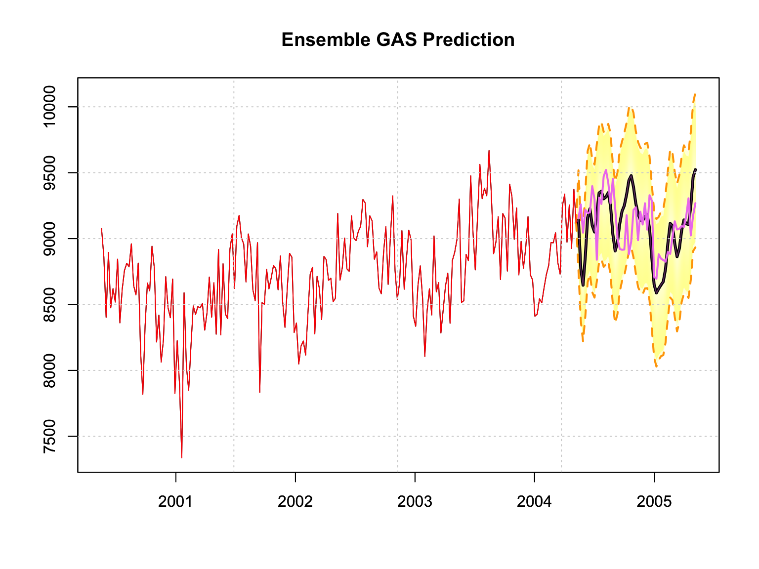

Some Additional Notes

Because the models were all estimated with the same transformation³, their state decompositions can also be ensembled. This could be particularly useful should custom views need to be incorporated into the prediction, which is usually done on the Trend component or the growth rate, allowing one to rebuild the full predictive distribution after intervening in some part of the state decomposition.

Conclusion

There should be no doubt about the value of ensembling. The key takeaway is: When in doubt, ensemble.

References

Harvey, Andrew, Siem Jan Koopman, and Jeremy Penzer. 1998. “Messy Time Series: A Unified Approach.” Advances in Econometrics 13: 103–44.

Pflug, Georg Ch, Alois Pichler, and David Wozabal. 2012. “The 1/n Investment Strategy Is Optimal Under High Model Ambiguity.” Journal of Banking & Finance 36 (2): 410–17.

Footnotes

See (Harvey, Koopman, and Penzer 1998)↩︎
After checking for equal sized prediction matrices in terms of samples and horizon.↩︎
No transformation, which is also equivalent to a Box Cox with lambda of 1.↩︎

Citation

BibTeX citation:

@online{galanos2022,
  author = {Galanos, Alexios},
  title = {Casting a Wide Net: Ensembling of Predictions},
  date = {2022-05-15},
  langid = {en}
}

For attribution, please cite this work as:

Galanos, Alexios. 2022. “Casting a Wide Net: Ensembling of Predictions.” May 15, 2022.