Code
# load required packages
library(tsmethods)
library(tsaux)
library(tsets)
library(xts)
library(tsdistributions)
library(data.table)
library(future.apply)
library(magrittr)
library(ggplot2)# load required packages
library(tsmethods)
library(tsaux)
library(tsets)
library(xts)
library(tsdistributions)
library(data.table)
library(future.apply)
library(magrittr)
library(ggplot2)Finding stable patterns in data is a key requirement if we are to have any success in forecasting the future. These patterns are identified by analyzing the historical behavior of data, and may include seasonal patterns, particular types of growth, fixed and moving holidays and know causal drivers. These can collectively be termed the signal, and the remainder as the noise. In estimating such signals, we usually make some assumptions about the structure of the noise. However, when the data is contaminated by anomalies which violate our assumptions, then it becomes increasingly difficult to cleanly identify the signals.
Large spikes in data series have typically been associated with the term outliers. These lead to clear contamination of normal process variation under most types of dynamics and is therefore the type of anomaly which is most general across different types of data generating mechanisms. While such spikes usually decay almost instantaneously, others may decay at a slower pace (temporary shifts) and some may even be permanent (level shifts). One generating mechanism for these anomalies if through a recursive AR(1) filter. The figure below shows an example of how such anomalies can be generated with different decay rates. The half-life of the decay of such shocks can be easily derived from the theory on ARMA processes and is equal to \(-\text{ln}\left(2\right)/\text{ln}\left(\alpha\right)\), where \(\alpha\) is the AR(1) coefficient. Thus, the closer this gets to 1, the closer the shock becomes permanent whereas a coefficient close to 0 is equivalent to an instantaneous decay.
x <- rep(0, 100)
x[50] <- 1
plot(filter(x, filter = 0, method = "recursive", init = 0), ylab = "", xlab = "")
lines(filter(x, filter = 0.5, method = "recursive", init = 0), col = 2, lty = 2)
lines(filter(x, filter = 0.8, method = "recursive", init = 0), col = 2, lty = 2)
lines(filter(x, filter = 1, method = "recursive", init = 0), col = 3, lty = 3, lwd = 2)
grid()
legend("topleft", c("Additive Outlier (alpha = 0.0)",
                    "Temporary Change (alpha = 0.5)",
                    "Temporary Change (alpha = 0.8)",
                    "Permanent Shift (alpha = 1.0)"), lty = c(1,2,2,3), bty = "n", col = c(1,2,2,3))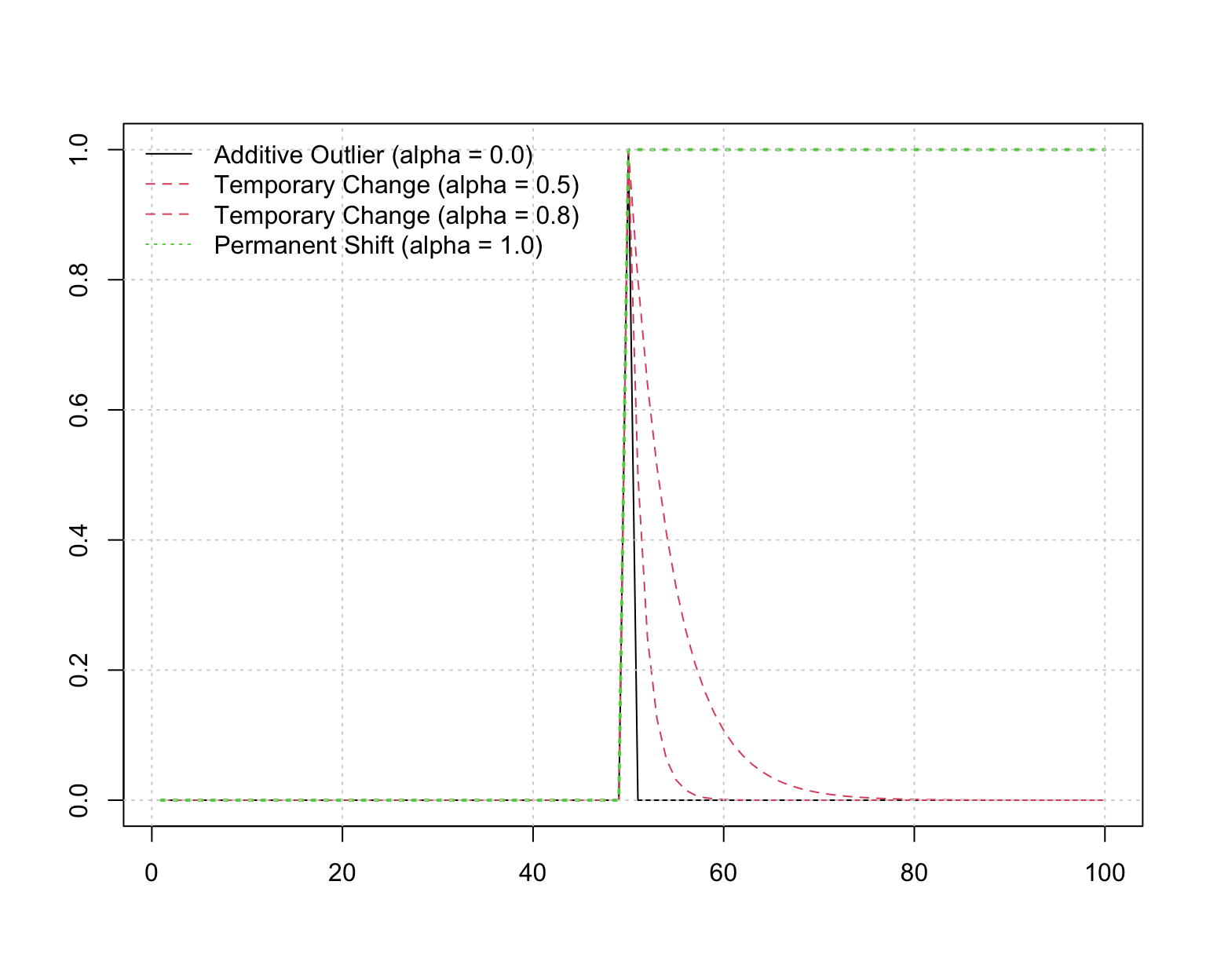
Sudden changes in the slope of the dynamics, may sometimes come about as a result of structural changes, such as technological innovation or other business changes. Such changes would technically fall under anomalies. However, there is another case which is based on the life cycle hypothesis of product adoption.1 When thinking of variance stabilizing transformations such as the Box-Cox, this is similar to changes in the \(\lambda\) parameter of the transformation. For instance, in the early stages of product adoption, we may observe exponential growth which may eventually stabilize to linear growth over time. Modelling the dynamics of such a process with standard models is likely to lead to poor long range forecasts. One interesting approach is provided in (Guo, Lichtendahl, and Grushka-Cockayne 2019).
Identifying different types of anomalies is usually undertaken as an integrated part of the assumed dynamics of the process. An established and flexible framework for forecasting economic time series is the state space model, or one of its many variants. For example, the basic structural time series model of (Harvey 1990) is a state of the art approach to econometric forecasting, decomposing a series into a number of independent unobserved structural components:
\[ \begin{aligned} y_t &= \mu_t + \gamma_t + \varepsilon_t,\quad &\varepsilon_t\sim N(0,\sigma)\\ \mu_t &=\mu_{t-1} + \beta_{t-1} + \eta_t,\quad &\eta_t\sim N(0,\sigma_\eta)\\ \beta_t &= \beta_{t_1} + \zeta_t,\quad &\zeta_t\sim N(0,\sigma_\zeta)\\ \gamma_t &= - \sum^{s-1}_{j=1}\gamma_{t-j} + \omega_t,\quad &\omega_t\sim N(0,\sigma_\omega)\\ \end{aligned} \tag{1}\]
which uses random walk dynamics for the level, slope and seasonal components, each with an independent noise component. Variations to this model include the innovations state space model which assumes fully correlated components and is observationally equivalent to this model but does not require the use of the Kalman filter since it starts from a steady state equilibrium and hence optimizing the log likelihood is somewhat simpler and faster.
In this structural time series representation, additive outliers can be identified by spikes in the observation equation; level shifts by outliers in the level equation; and a large change in the slope as an outlier in the slope equation (and similar logic applies to the seasonal equation). Therefore, testing for such outliers in each of the disturbance smoother errors of the models can form the basis for the identification of anomalies in the series.2
Direct equivalence between a number of different variations of this model and the more well known ARIMA model have been established. In the ARIMA framework, a key method for the identification of anomalies is based on the work of (Chen and Liu 1993), and is the one we use in our approach.3 This approach uses multi-pass identification and elimination steps based on automatic model selection to identify the best anomaly candidates (and types of candidates) based on information criteria. This is a computationally demanding approach, particularly in the presence of multiple components and long time series data sets. As such, we have implemented a slightly modified and faster approach, as an additional option, which first identifies and removes large spikes using a robust STL decomposition and MAD criterion, then deseasonalizes and detrends this cleaned data again using a robust STL decomposition, before finally passing the irregular component to the method of (Chen and Liu 1993), as implemented in the tsoutliers package. Finally, the outliers from the first stage are combined with the anomalies identified in the last step (and duplicates removed), together with all estimated coefficients on these anomalies which can then be used to clean the data. The tsaux package provides 2 functions: auto_regressors automatically returns the identified anomalies, their types and coefficients, whilst auto_clean automatically performs the data cleaning step. The functions allow for the use of the modified approach as well as the direct approach of passing the data to the tso function.
One shortcoming of the current approach is that for temporary change identification, the AR coefficient defaults to 0.7 and there is no search performed on other parameters. Adapting the method to search over different values is left for future research.
We start with an illustration of data contamination. Starting with a simulated series of level + slope, we then proceed to contaminate it with outliers, temporary changes and level shifts.
set.seed(10125)
y <- tsets:::ets_sample(model = "AAN", h = 52*5, alpha = 0.25, beta = 0.01,
                        gamma = 1e-12, sigma = 10,
                        seed_states = c("l0" = 100, "b0" = 1))
y <- y$Simulated
par(mfrow = c(4, 1), mar = c(3,3,3,3))
plot(as.zoo(y), main = "Original", ylab = "", xlab = "")
grid()
y_contaminated <- y %>% additive_outlier(time = 25, parameter = 1)
plot(as.zoo(y_contaminated), main = "+Additive Outlier[t=25]",  ylab = "", xlab = "")
grid()
y_contaminated <- y_contaminated %>% temporary_change(time = 120, parameter = 0.75, alpha = 0.7)
plot(as.zoo(y_contaminated), main = "+Temporary Change[t=120]",  ylab = "", xlab = "")
grid()
y_contaminated <- y_contaminated %>% level_shift(time = 200, parameter = -0.25)
plot(as.zoo(y_contaminated), main = "+Level Shift[t=200]",  ylab = "", xlab = "")
grid()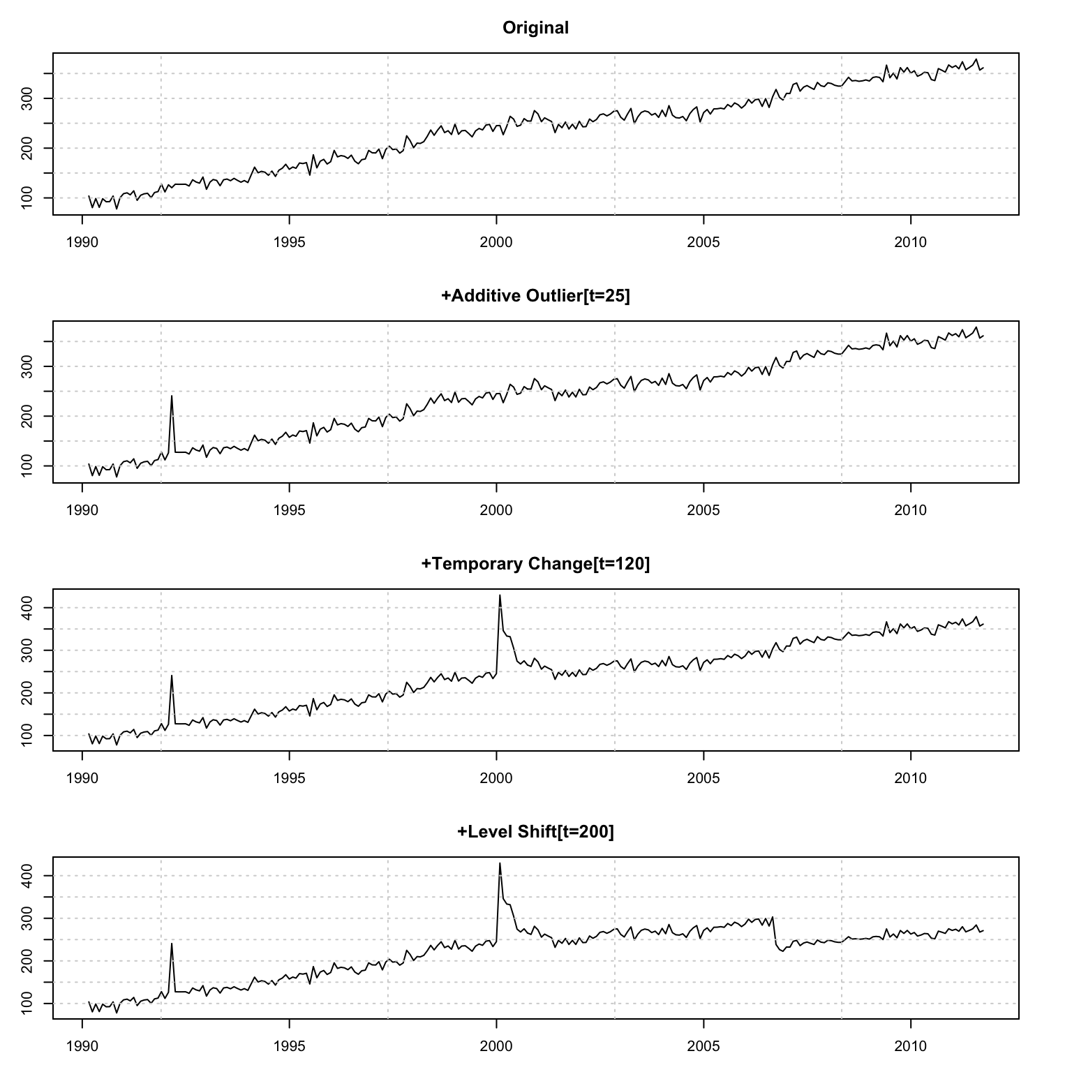
We now pass the contaminated series to the anomaly identification function auto_regressors. The tso function directly identifies the correct number, timing and types of anomalies.4
xreg <- auto_regressors(y_contaminated, frequency = 52,
                        return_table = TRUE,
                        auto_arima_opts = list(seasonal = FALSE), method = "full")
xreg[,time := which(index(y_contaminated) %in% xreg$date)]
print(xreg)
## Index: <type>
## type date filter coef time
## <char> <Date> <num> <num> <int>
## 1: AO 1992-02-29 0.0 118.81429 25
## 2: TC 2000-01-31 0.7 174.45303 120
## 3: LS 2006-09-30 1.0 -65.82534 200While we can call directly the auto_clean function, we’ll instead show how to use the returned table to decontaminate the data.
x <- cbind(additive_outlier(y_contaminated, time = xreg$time[1], add = FALSE),
           temporary_change(y_contaminated, time = xreg$time[2], alpha = xreg$filter[2],
                            add = FALSE),
           level_shift(y_contaminated, time = xreg$time[3], add = FALSE))
x <- x %*% xreg$coef
y_clean <- y_contaminated - x
par(mfrow = c(2,1), mar = c(3,3,3,3))
plot(as.zoo(y_contaminated), main = "Anomaly Decomtanination", xlab = "", ylab = "")
lines(as.zoo(y_clean), col = 2, lty = 2, lwd = 2)
lines(as.zoo(y), col = 3, lty = 3, lwd = 2.5)
grid()
legend("topleft", c("Contaminated", "Clean", "Original"), col = 1:3, bty = "n", lty = 1:3)
plot(zoo(x, index(y)), main = "Anomalies", xlab = "", ylab = "")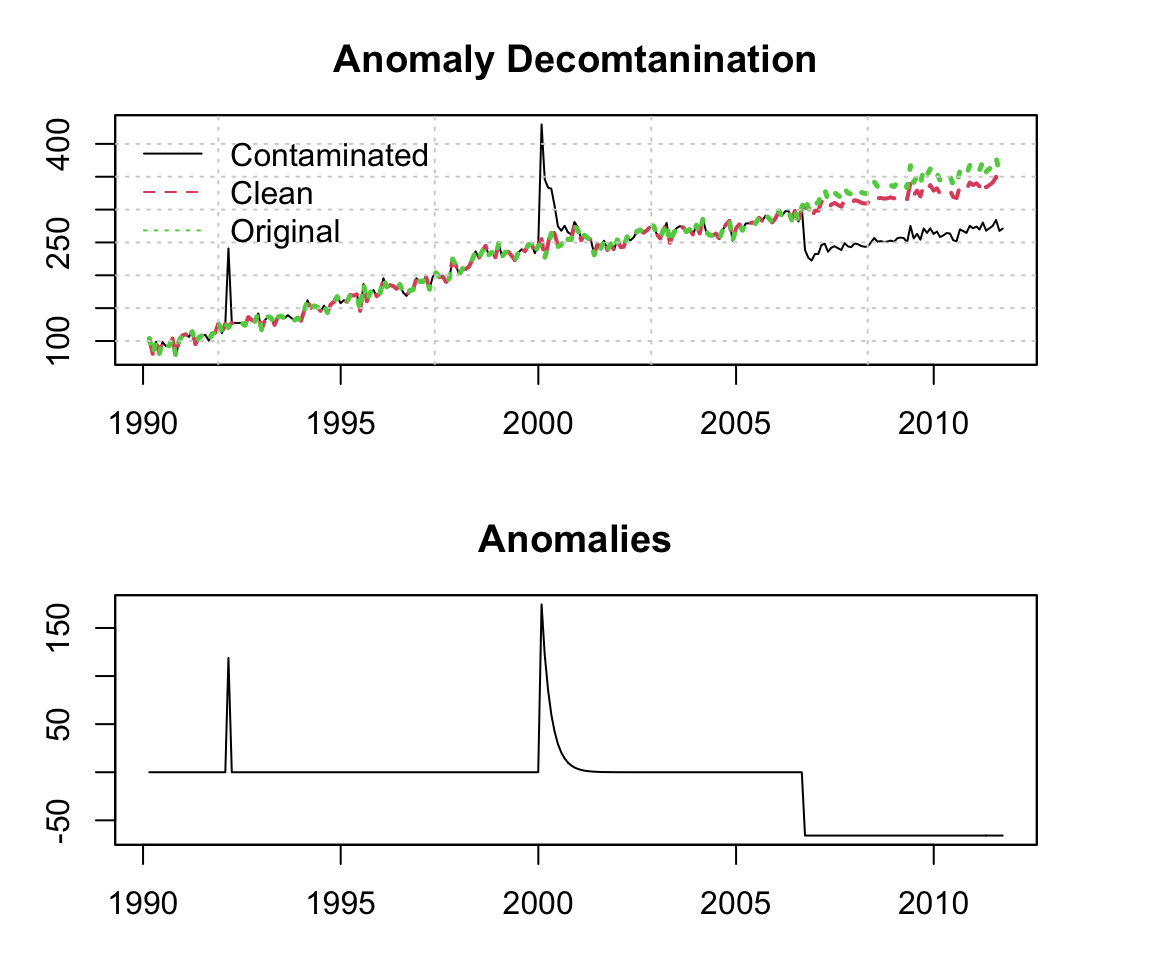
Next, we perform a simulation exercise to see how well the method works on a series with anomalies arriving at random times. To keep things simple, we contaminate the series with 4 additive outliers and 2 temporary changes, all arriving at random times with random coefficients. There are two key ways to measure the performance of this simulation; the very detailed looks at measuring the correct number, type and and timing of anomalies; the other way is to simply measure the goodness of fit of the decontaminated series against the original series. We choose the latter since the detailed method requires writing a lot of coding for matching which is not conducive to a blog post. We measure goodness of fit using MAPE since it’s simple and explainable. It should be noted that this is a purely artificial example, since most real data is much more noisy and can contain anomalies which happen at or near the same time point.
plan(multisession)
simulation <- future_lapply(1:1000, function(i){
 random_parameters <- runif(6, 0.3, 0.8)
 random_times <- sample(2:((52*5) - 1), 6, replace = FALSE)
 y_contaminated <- y %>% additive_outlier(time = random_times[1], parameter = random_parameters[1]) %>%
  additive_outlier(time = random_times[2], parameter = random_parameters[2]) %>%
  additive_outlier(time = random_times[3], parameter = random_parameters[3]) %>%
  additive_outlier(time = random_times[4], parameter = random_parameters[4]) %>%
  temporary_change(time = random_times[5], parameter = random_parameters[5]) %>%
  temporary_change(time = random_times[6], parameter = random_parameters[6])
 y_clean <- try(auto_clean(y_contaminated, frequency = 52, maxit.iloop = 20, maxit.oloop = 20, types = c("AO","TC"),
                       auto_arima_opts = list(seasonal = FALSE), method = "full", cval = 3.5, check.rank = T), silent = TRUE)
 if (inherits(y_clean,'mod-error')) {
  stat <- as.numeric(NA)
 } else {
  if (NROW(na.omit(y_clean)) != NROW(y)) {
   stat <- as.numeric(NA)
  } else {
   stat <- mape(y, y_clean)
  }
 }
  return(data.table(sim = i, mape = stat))
}, future.seed = TRUE, future.packages = c("tsets","tsaux","xts","data.table","magrittr"))
plan(sequential)
simulation <- rbindlist(simulation)ggplot(simulation, aes(x = mape*100)) +
geom_density(adjust = 2, alpha = 0.5, fill = "orange", colour = NA) +
ggthemes::theme_pander() + ylab("") +
xlab("Goodness of Fit (%MAPE)") + ggtitle("Decontaminated Series")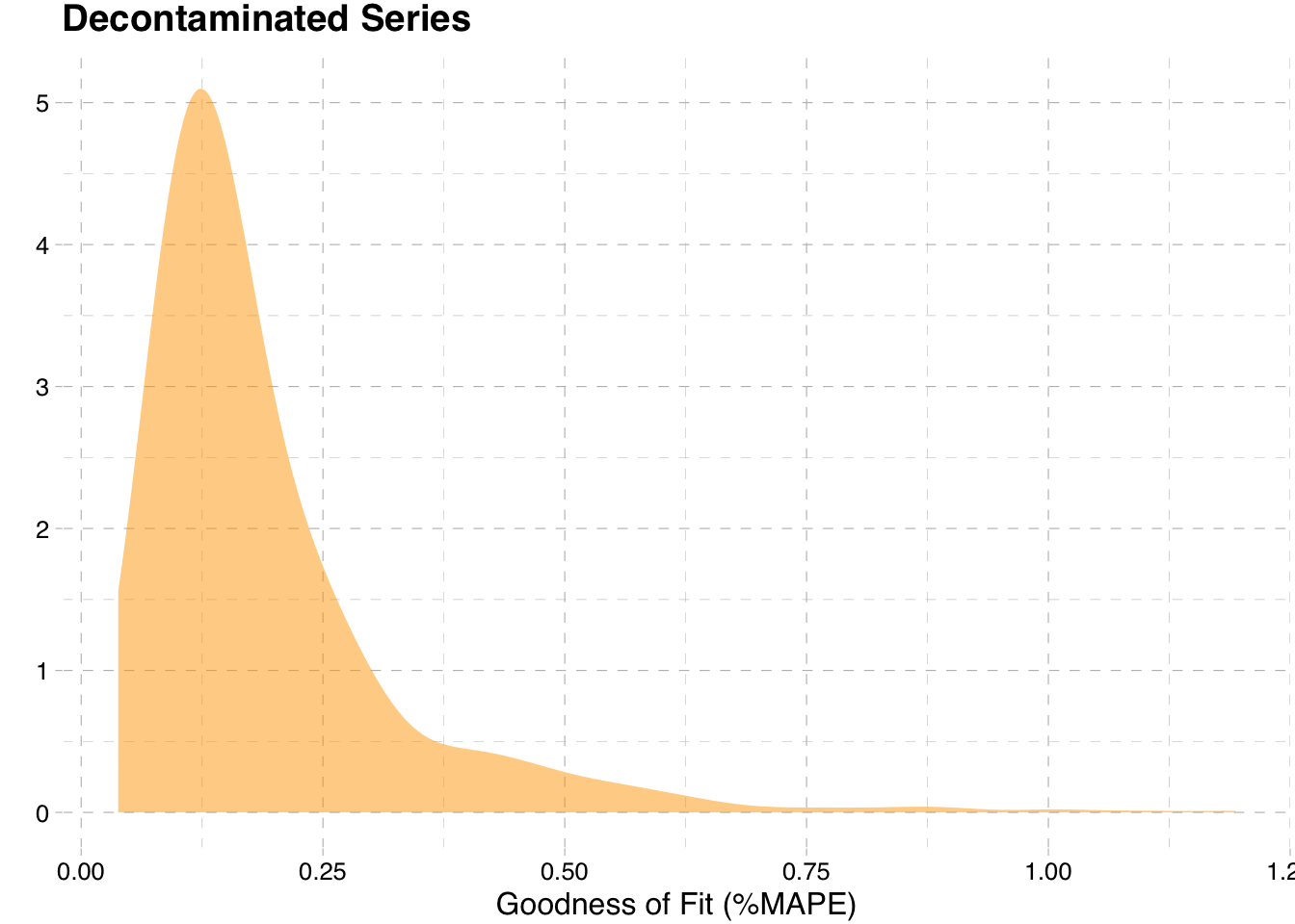
The very low MAPE we observe overall provides clear evidence that the detection algorithm performs quite well in eliminating the anomalies to the point where the decontaminated data is almost identical to the original series.
For the purpose of forecasting, level shifts should never be used in the anomaly cleaning step. Once the level is changed by such a structural shift, it forever changed and we are usually interested in forecasting from current levels rather than the some counter factual level (unless there is a specific reason to do so). However, they can be included as part of a model’s regressors in order to reduce the variance of the noise.
In some cases, we may be interested in incorporating the uncertainty of future anomalies in the data.5 There are many ways to address this, but here we consider a change of distribution by infusing non-normal errors into the predict function. The example below illustrates how to use a skewed and heavy tailed distribution. This leaves the standard deviation of the decontaminated model intact, but allows for fatter tails and skewness. However, it would also be possible to simply change the standard deviation to a higher value and continue to use the Normal distribution.
set.seed(12111)
random_parameters <- runif(6, 0.5, 1)
 random_times <- sample(2:((52*5) - 1), 6, replace = FALSE)
 y_contaminated <- y %>% additive_outlier(time = random_times[1], parameter = random_parameters[1]) %>%
  additive_outlier(time = random_times[2], parameter = random_parameters[2]) %>%
  additive_outlier(time = random_times[3], parameter = random_parameters[3]) %>%
  additive_outlier(time = random_times[4], parameter = random_parameters[4]) %>%
  temporary_change(time = random_times[5], parameter = random_parameters[5]) %>%
  temporary_change(time = random_times[6], parameter = random_parameters[6])
 y_clean <- try(auto_clean(y_contaminated, frequency = 52, maxit.iloop = 20, maxit.oloop = 20, types = c("AO","TC"),
                       auto_arima_opts = list(seasonal = FALSE), method = "full", cval = 3.5, check.rank = T), silent = TRUE)
model_contaminated <- estimate(ets_modelspec(y_contaminated, model = "AAN", frequency = 52))
model_clean <- estimate(ets_modelspec(y_clean, model = "AAN", frequency = 52))
nig_distribution <- estimate(distribution_modelspec(scale(residuals(model_contaminated, raw = TRUE)),
                                                    distribution = "nig"))
r <- rdist("nig", n = 5000 * 52, mu = 0, sigma = 1,
           skew = coef(nig_distribution)["skew"], shape = coef(nig_distribution)["shape"])
r <- matrix(r, ncol = 52, nrow = 5000)
p_clean_nig <- predict(model_clean, h = 52, nsim = 5000, innov = r, innov_type = "z")
p_clean_norm <- predict(model_clean, h = 52, nsim = 5000)par(mar = c(3,3,3,3), mfrow = c(1,1))
plot(p_clean_nig, gradient_color = "white", interval_color = "steelblue",
interval_quantiles = c(0.005, 0.995), interval_type = 1,
main = "Prediction [99% Coverage]")
plot(p_clean_norm$distribution, interval_color = "orange",
interval_quantiles = c(0.005 , 0.995), add = TRUE, interval_type = 1)
lines(index(y), as.numeric(y_contaminated), col = 3)
legend("topleft", c("Clean|Series","Contaminated|Series",
"Prediction|NIG","Prediction|Norm"),
col = c("red","green","steelblue","orange"), lty = 1, bty = "n")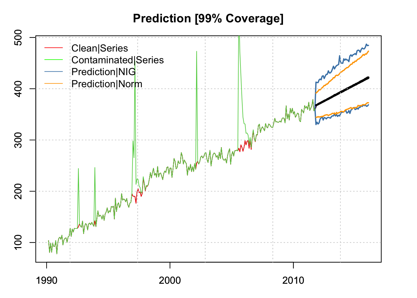
With 99% coverage. we can see that the NIG distributed errors provide for heavier tails, skewed towards positive shocks, which is what we observed given the way we generated the anomalies (to be positive).
Anomalies contaminate process dynamics with noise which is not part of normal variation. This make it difficult to extract clean signals and should therefore be addressed as part of any forecasting strategy. This should be distinct from how one thinks about future uncertainty which can be addressed separately.
see (De Jong and Penzer 1998).↩︎
The approach used in the tsaux package calls the tso function in the tsouliers package.↩︎
This may not always be the case depending on the amount of noise and other artifacts in the underlying series and the size of the anomalies versus normal process noise.↩︎
An example would be forecasting for peaks.↩︎
@online{galanos2022,
  author = {Galanos, Alexios},
  title = {Messy Data and Anomaly Detection},
  date = {2022-05-16},
  url = {https://www.nopredict.com/blog/posts/2022-05-15-messy-data-and-anomaly-detection/},
  langid = {en}
}